How I built a scraper to measure activity of MPs
October 03, 2016
When the president of the parliament states that there are some MPs “doing nothing” you know what to do as a data journalist: you turn to the numbers. This is how I did that and how I got a scatter plot in a printed paper and an interactive one online.
The data
I knew that the Flemish parliament has a strong open data policy and publishes all parliamentary activities of the members of parliament, so I decided to check out their API. But the API proved to be a bit difficult for me:
- To get the info I was interested in, I had to make a lot of API calls, store the results and make a lot of other API calls.
- The response file formats are json and xml. I don’t have a lot of experience getting data out of these formats and this proved to be challenging.
After a while I gave up on the API, the xml’s and the json’s and I decided to just scrape the website instead. Luckily, the website is very well structured and contains all the information I wanted in a very structured way.
I used the rvest R package for scraping. I took some time in the summer to learn R and some of its useful packages. I’m very glad I did that: it is paying off already.
What the scraper does (you can find all the code at the bottom of this page):
- It visits the page where all the MPs are listed and stores their names, the party they belong to and the urls of their personal profile pages.
- It then goes to all the profile pages and collects the urls to the pages where the activity of the MPs are listed (questions they asked, things they said in parliament and proposals they made).
- It then changes a parameter in these url’s to filter out the activity of only the current term.
- It visits the urls with the filter and gets the number of activities listed on these pages.
Fairly simple, all in all. I wasted much more time trying to collect the data with the API then writing the html scraper.
Then what?
I decided to analyse two measures: how much an MP said something in parliament and how many official documents (proposals, amendments, …) they filed. An obvious choice then was to make a scatter plot. I used ggplot2, another great R package I learned to work with, to do that.
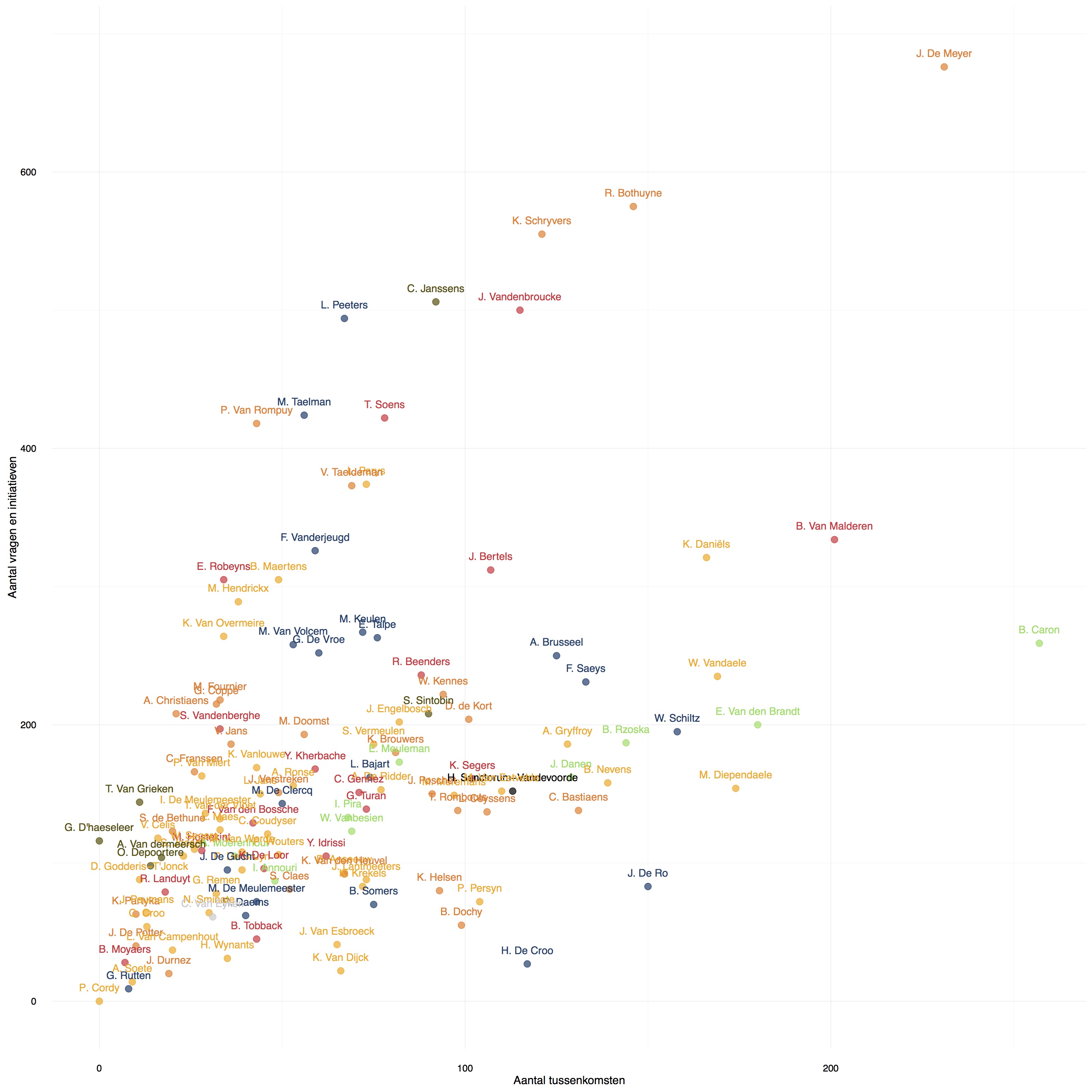
A clear trend, but also with some outliers in all directions: not bad for building a story. But how to do it?
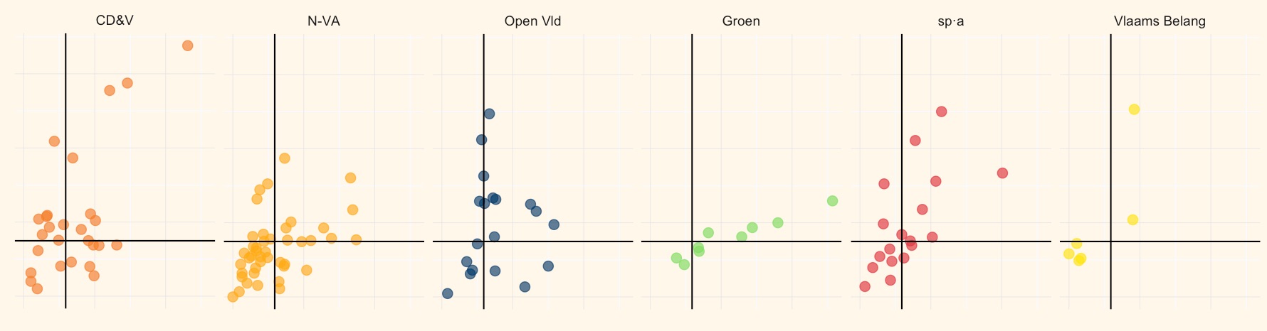
Key was to add lines for both medians. This divides the plot into 4 quadrants and I used these quadrants to classify the MPs as Busy Bees (a lot of interventions in parliament, a lot of documents filed), Silent Workers (few interventions, lot of docs), Chatterers (lot of interventions, few docs) and the Passive MPs (few interventions and few docs).
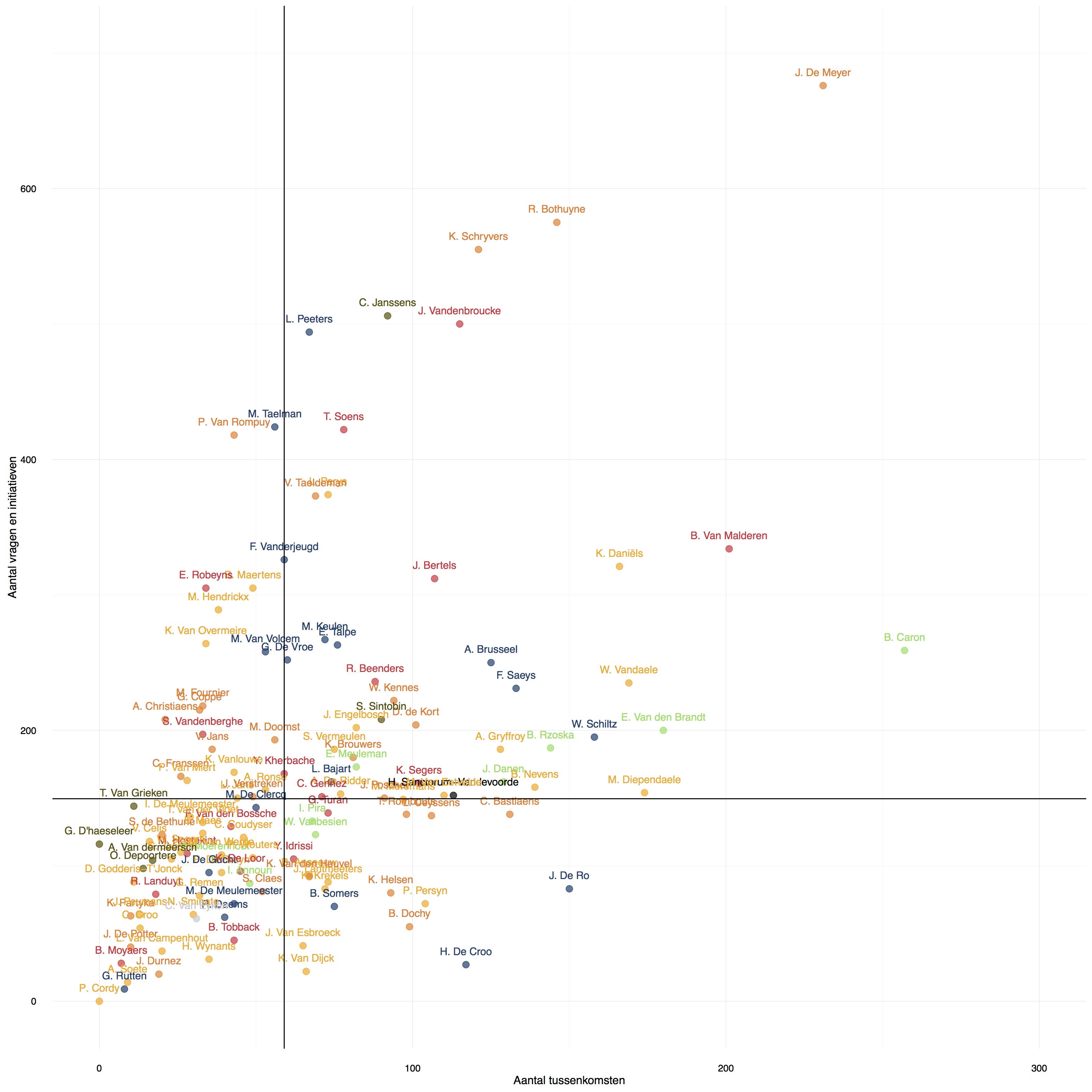
This added layer of classification, both in the story and in the graphic, proved to be the sugar to let the dry graphic that a scatter plot is to a lot of people (not to me!) go down. Without it, I don’t think I could have convinced the editors to run the graphic and I think a lot of people would have a harder time getting the chart.
Output
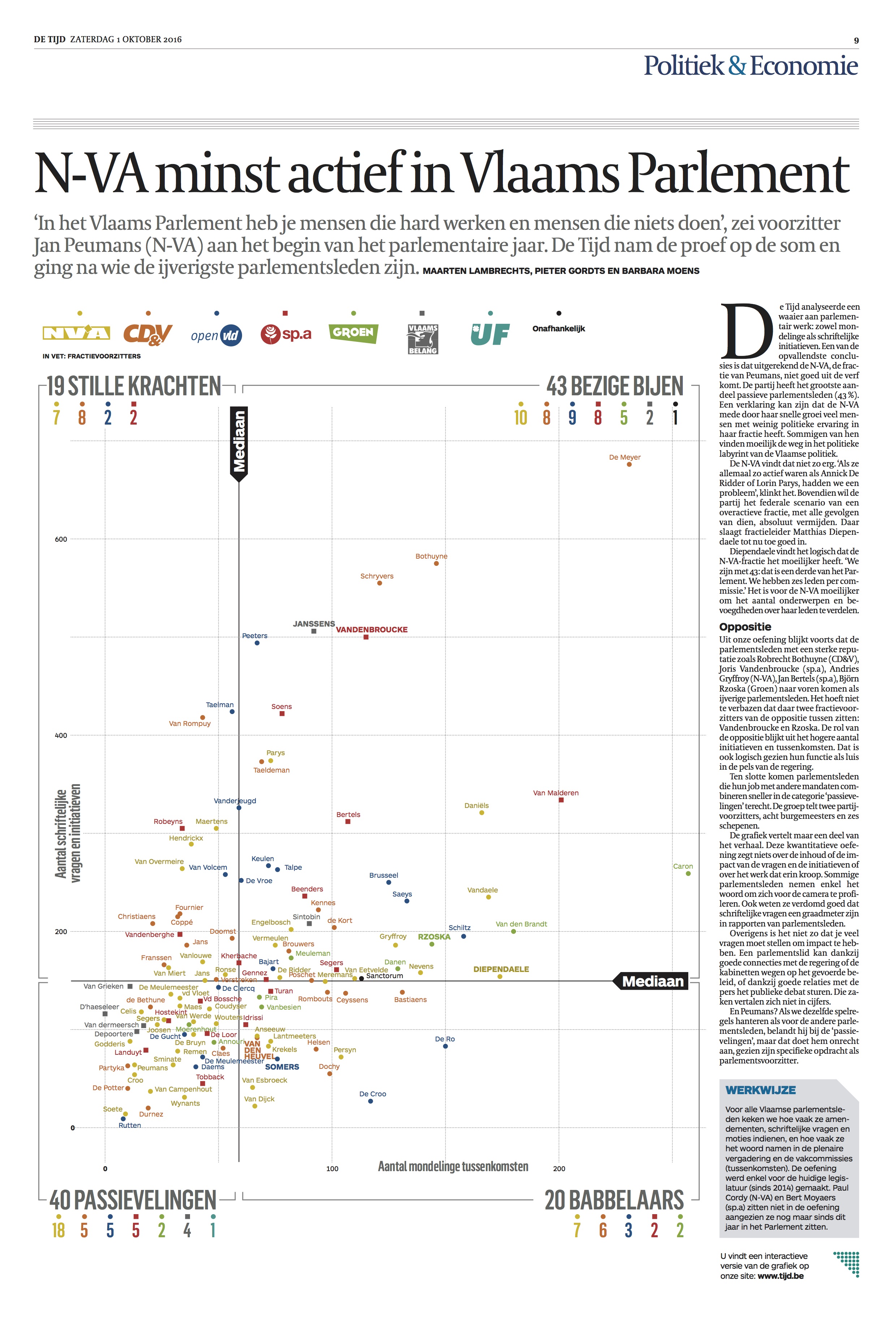
For print, I generated the scatter plot with ggplot2 and exported it as a pdf. Further processing for print (which involved the manual placement of the overlapping labels) was done by my colleague @filipysenbaert, reporting was done by 2 colleagues of the politics desk.
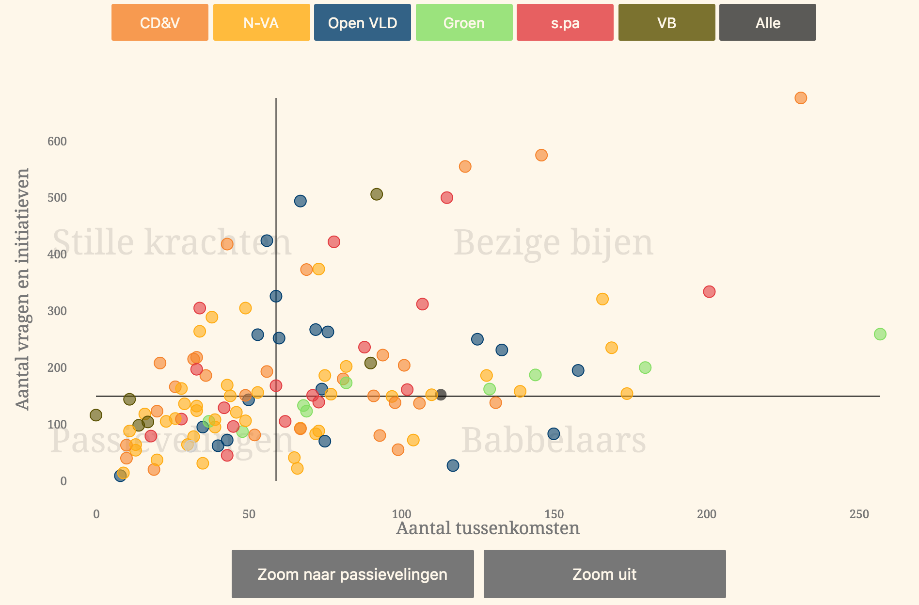
For the online version, I used D3 to make a scatter plot with buttons for highlighting and for zooming in on the ‘passive’ zone of the plot. Details of every MP are shown on hover/tap.
Mobile readers only get a static scatter plot, but they still get the small multiples for comparing the parties in parliament. Those were also generated with ggplot2.
R
As I wrote already: learning R payed off. And not only for getting the data and visualizing it: I now have an R script (see below) that I can run by clicking a button and it will get all the data, put it in the right format, visualize it and prepare the data for the interactive scatter plot. No tedious manual editing anymore!
I actually edited the script and ran it on Friday morning (the graphic was published on Saturday). Getting new data while I still had a lot of work to do for publishing was something I would have never done if there were some manual steps involved in the data gathering and processing.
Bonus: explaining the median
I always struggle to explain in words what the median means exactly. But graphically this is surprisingly easy: on the scatter plot half of the points are always above, below left and right of the black lines. Can’t be easier, I think.
The code
So here is the code you need to get all the data and make the plots:
library(rvest)
library(ggplot2)
library(tidyr)

vlaverturl <- "https://www.vlaamsparlement.be/vlaamse-volksvertegenwoordigers"
vlaverthtml <- read_html(vlaverturl)

##Get the names, parties and the urls of the profile pages
vlavert <- vlaverthtml %>% html_nodes(".field--name-volledige-naam") %>% html_text()
vlapart <- vlaverthtml %>% html_nodes(".field--name-huidigefractie") %>% html_text()
vlaverturls <- vlaverthtml %>% html_nodes("span a") %>% html_attr("href")

rawdata <- data.frame()
index <- 0

##Go to the profile pages of all the MP's and collect the data
base_verturl <- "https://www.vlaamsparlement.be"

for(verturlid in vlaverturls){
  print(index)
  index <- index + 1

  verturl <- paste(base_verturl,verturlid,sep="")
  verthtml <- read_html(verturl)

  ##Initiatieven
  vertiniturl <- verthtml %>% html_node(".field--name-recent-documents-link .field__items .field__item a") %>% html_attr("href")
  vertiniturl <- sub("publicatiedatum[van][date]=all","publicatiedatum[van][date]=current_legislature", vertiniturl, fixed = TRUE)
  initiatieven <- read_html(paste(base_verturl, vertiniturl, sep="")) %>% html_node("h1.page-title") %>% html_text()

  ##Vragen
  vertvragenurl <- verthtml %>% html_node(".field--name-recent-questions-link .field__items .field__item a") %>% html_attr("href")
  vertvragenurl <- sub("publicatiedatum[van][date]=all","publicatiedatum[van][date]=current_legislature", vertvragenurl, fixed = TRUE)
  vragen <- read_html(paste(base_verturl, vertvragenurl, sep="")) %>% html_node("h1.page-title") %>% html_text()

  ##Tussenkomsten
  verttussenkurl <- verthtml %>% html_node(".field--name-recent-interventions-link .field__items .field__item a") %>% html_attr("href")
  verttussenkurl <- sub("publicatiedatum[van][date]=all","publicatiedatum[van][date]=current_legislature", verttussenkurl, fixed = TRUE)
  tussenkomsten <- read_html(paste(base_verturl, verttussenkurl, sep="")) %>% html_node("h1.page-title") %>% html_text()

  vertdata <- data.frame()
  vertdata <- data.frame(vlavert[index], vlapart[index], initiatieven, vragen, tussenkomsten, vlaverturls[index])

  rawdata <- rbind(rawdata, vertdata)
}

colnames(rawdata) <- c("naam", "partij", "initiatieven", "vragen", "tussenkomsten", "url")

finaldata <- rawdata
##Remove text we don't need
finaldata$initiatieven <- sub("Ongeveer ", "", finaldata$initiatieven, fixed=TRUE)
finaldata$initiatieven <- sub(" zoekresultaten in de huidige zittingsperiode", "", finaldata$initiatieven, fixed=TRUE)
finaldata$vragen <- sub("Ongeveer ", "", finaldata$vragen, fixed=TRUE)
finaldata$vragen <- sub(" zoekresultaten in de huidige zittingsperiode", "", finaldata$vragen, fixed=TRUE)
finaldata$tussenkomsten <- sub("Ongeveer ", "", finaldata$tussenkomsten, fixed=TRUE)
finaldata$tussenkomsten <- sub(" zoekresultaten in de huidige zittingsperiode", "", finaldata$tussenkomsten, fixed=TRUE)

##Convert to numbers
finaldata$initiatieven <- as.integer(finaldata$initiatieven)
finaldata$vragen <- as.integer(finaldata$vragen)
finaldata$tussenkomsten <- as.integer(finaldata$tussenkomsten)

##Format names and ad questions and initiatives
finaldata <- finaldata %>% separate(naam, c("voornaam", "achternaam"), " ", extra = "merge")
finaldata$initiaal <- paste(substr(finaldata$voornaam, 1, 1), ".", sep="")
finaldata$initnaam <- paste(finaldata$initiaal, finaldata$achternaam, sep=" ")
finaldata$vrageninitiatieven <- finaldata$vragen + finaldata$initiatieven

median.tussenkomsten <- median(finaldata$tussenkomsten)
median.vrageninitiatieven <- median(finaldata$vrageninitiatieven)

finaldata <- select(finaldata, voornaam, achternaam, initiaal, initnaam, partij, initiatieven, vragen, tussenkomsten, vrageninitiatieven, profiel, url)

write.csv(finaldata, file="finaldata_30-09.csv", row.names = FALSE)

scatter <- ggplot(finaldata, aes(x = tussenkomsten, y = vrageninitiatieven, col = partij)) + geom_point( alpha = 0.7, size = 3) + theme_minimal() + geom_text(aes(label = initnaam), nudge_y = 10) + scale_colour_manual(values = c("#83de62","#ffac12", "#003d6d", "#f5822a", "#e23a3f", "#5a5101", "#000000", "#cccccc")) + labs(x = "Aantal tussenkomsten", y = "Aantal vragen en initiatieven") + theme(legend.position="none") + geom_hline(aes(yintercept=median.vrageninitiatieven)) + geom_vline(aes(xintercept=median.tussenkomsten))
##+ scale_x_continuous(limit = c(0, 300)) + scale_y_continuous(limit = c(0, 700))

scattergrid <- ggplot(finaldata, aes(x = tussenkomsten, y = vrageninitiatieven, col = partij)) + geom_point( alpha = 0.2, size = 3) + theme_minimal() + scale_colour_manual(values = c("#83de62","#ffac12", "#003d6d", "#f5822a", "#e23a3f", "#ffe500", "#000000", "#cccccc")) + labs(x = "Aantal tussenkomsten", y = "Aantal vragen en initiatieven") + theme(legend.position="none") + geom_hline(aes(yintercept=median.vrageninitiatieven)) + geom_vline(aes(xintercept=median.tussenkomsten)) + facet_grid(. ~ partij) + theme(panel.background = element_rect(fill = '#fef7ea', colour = '#fef7ea'), plot.background = element_rect(fill = '#fef7ea', colour = '#fef7ea'))