The Herds of Europe

I immediately fell for Jonas Schöley’s European population bubble grid map when I first saw it:

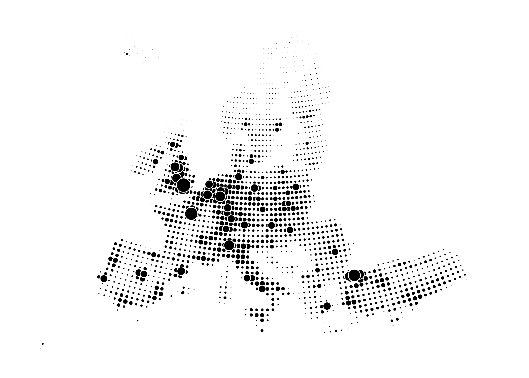
As he describes in his introductory blog post, part of Jonas’ motivation to make this map was to use areas to show magnitude instead of color, like is the case in a standard choropleth. Another advantage of this map type is that it smooths out the effect of sometimes arbitrary and very irregular administrative boundaries. That is why I think bubble grid maps are a very good alternative to choropleths when you want to show a broad overview of the geographical distribution of a variable.

Another motivation for Jonas to make this kind of map was to ‘just mess around with R, the eurostat and sf packages.’ I was just preparing to get my feet wet with the (relatively) new sf package, a package to work with geographical data in R that integrates nicely with the latest version of the visualisation package ggplot2. So this was an excellent opportunity for me to dive in. Luckily, Jonas shared his very well documented R code on his site, so I had a very good starting point.

As I was already messing around with domestic animal data, I decided to visualise the geography of European domestic animal herds. So here are the cows, pigs, sheep, goats and buffaloes of Europe! You can find the R code I used at the bottom of this page.

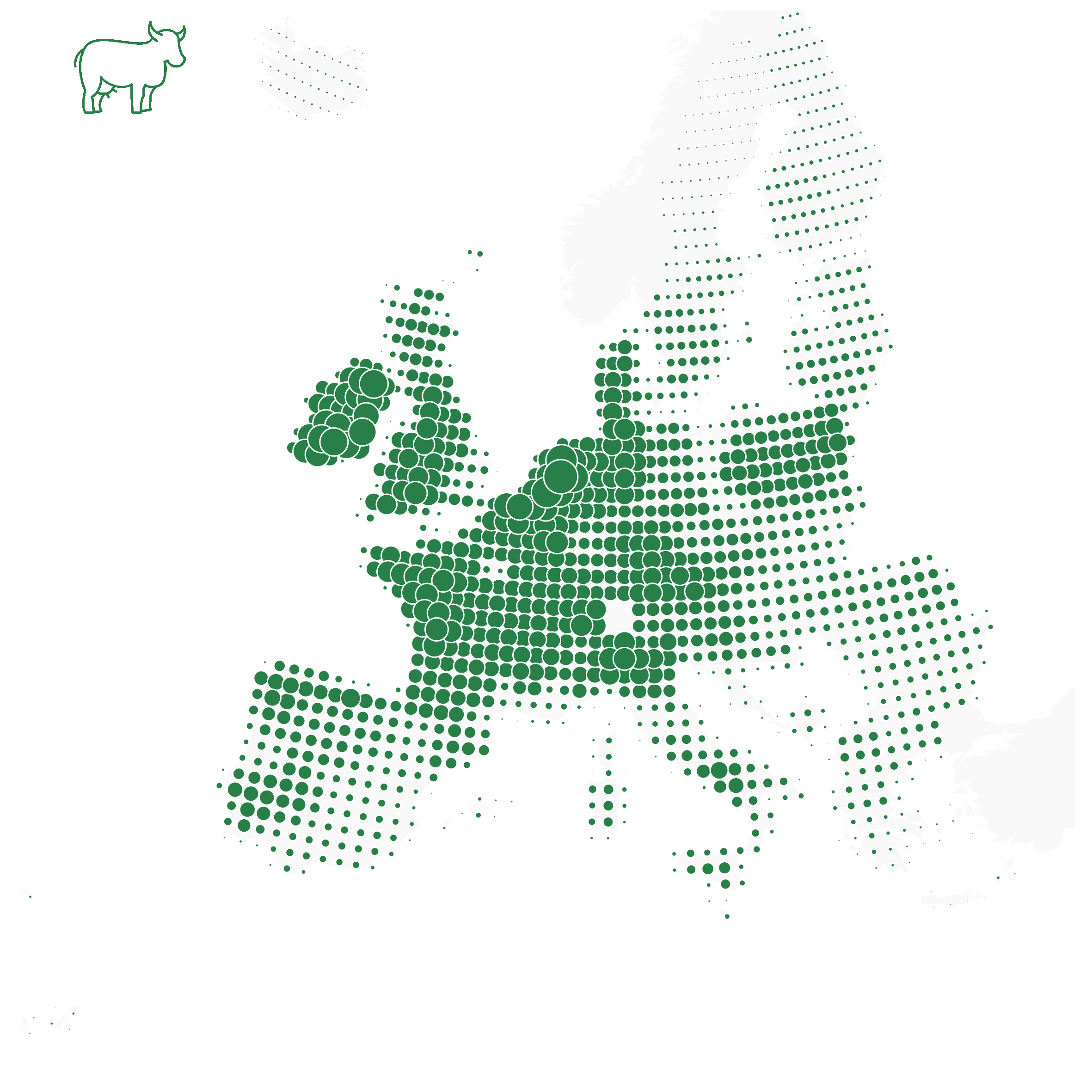
Cows

Cows are quite evenly distributed across Europe (compare their distribution to the much more clustered human population on the map above). You can notice a lack of green dots in the north and center of Europe: those are Norway, Switzerland and the Balkan countries, non-EU countries for which Eurostat (where I took the data from) doesn’t publish any data for. I definitely hope the cows from the UK will not disapear from this map next year too. Also notice how Paris is digging a almost cowless hole into western Europe.

Pigs

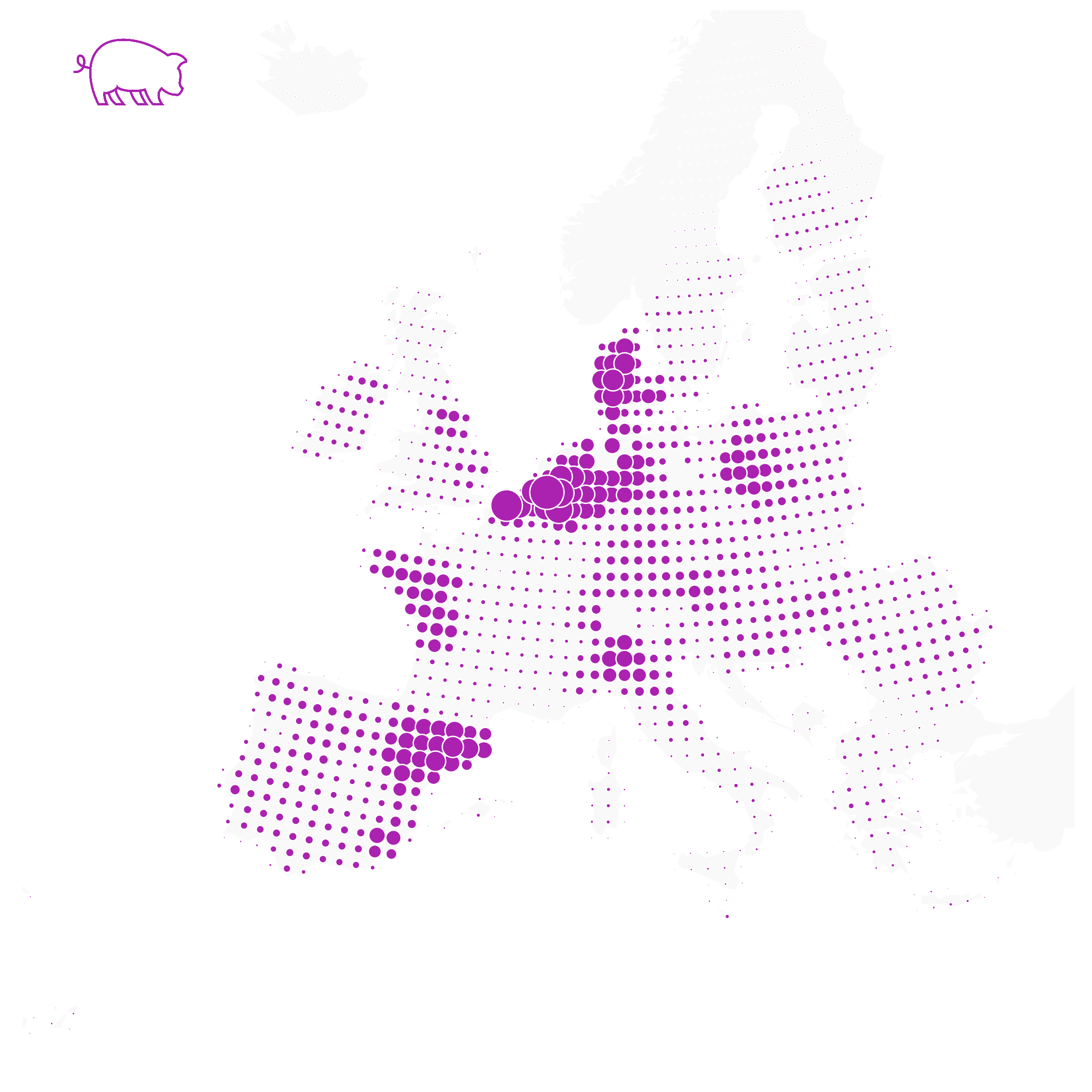
The European distribution of pigs is much more regionally concentrated. Intensive pig breeding is found primarily in Flanders (the northern part of Belgium, where I live), the Netherlands and Denmark. Pig farms there are typically located not too far away from big ports, through which protein rich fodder, like soy beans is imported. This allows pig breeders to raise pigs without having any or much agricultural land: pigs are bred inside and fed with imported fodder. (The problem then becomes having to much manure, no joke)

More intensive pig breeding is also found in northwestern France and Catalonia. You can also see where your jamón and prosciutto are coming from.

Buffaloes

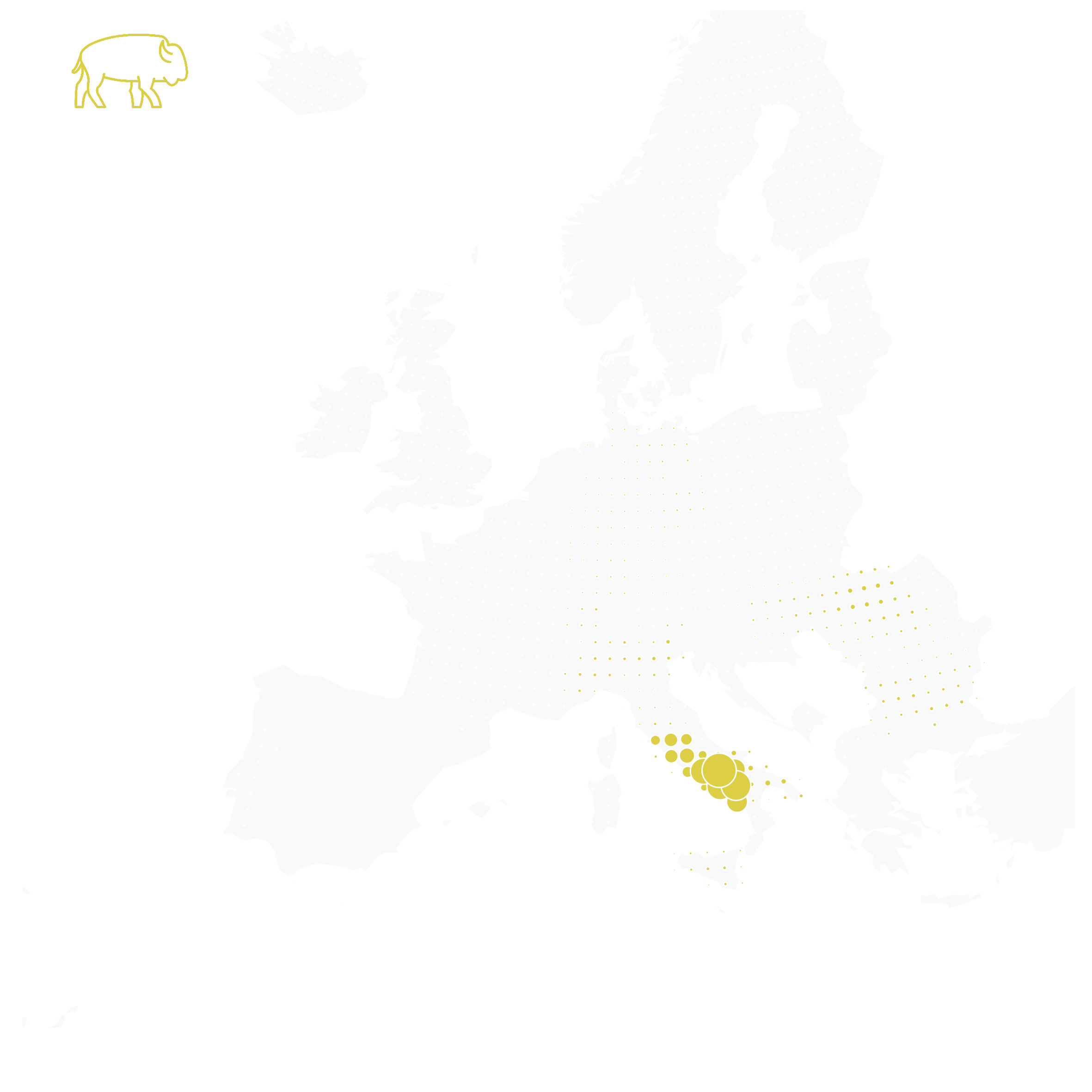
What? Buffalo breeding in Europe? Of course, where do you think your Mozzarella di bufala comes from?

Sheep

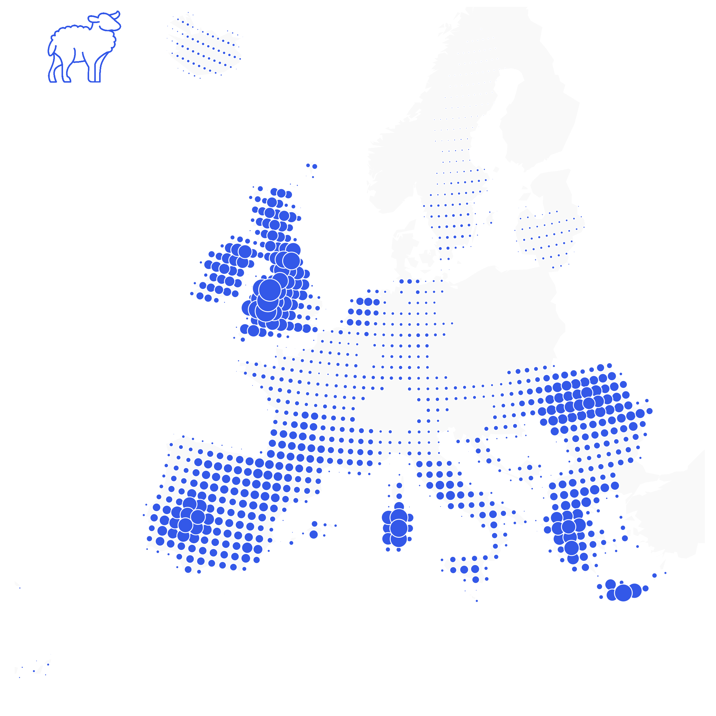
Europe’s sheep breeding ‘capital’ is clearly England. But other notable sheep regions are southwestern Spain (Manchego!), Corsica, Greece (Feta!) and Hungary-Romania.

Please notice that the gaps in the data for sheep stretch further then the non-EU countries: sheep data for Poland and Slovenia were also lacking.

Goats

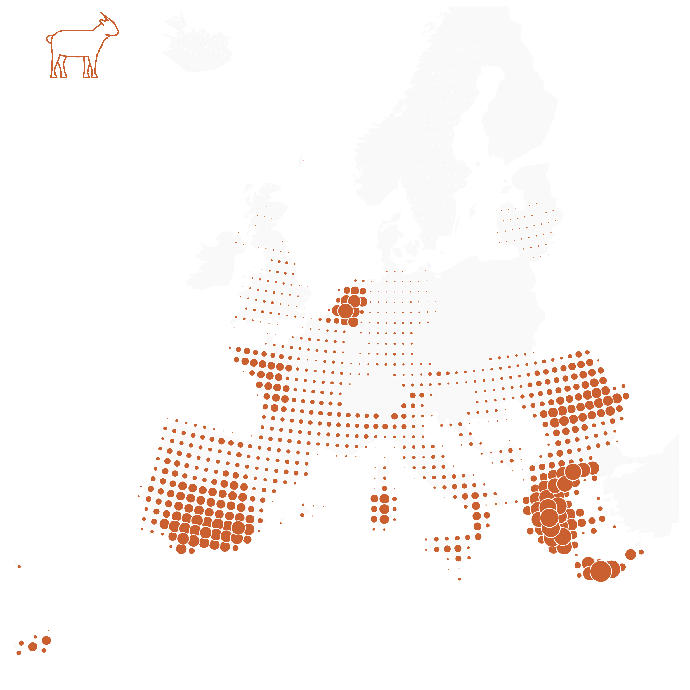
Like sheep, goats are very prevalent in Greece. But goat breeding is also common in southern Spain, western France and the Netherlands. And check how goats make the Canary Islands visible on the map for the first time.

Code

Below, you can find the code to generate these maps. Make sure you have at least version 3 of ggplot2 installed (otherwise geom_sf() will not work). Kudos to Jonas for sharing his code.

library(eurostat)  # eurostat data
library(dplyr) # tidy data transformation
library(sf)        # simple features GIS
library(lwgeom)
library(ggplot2)
library(png)

#NUTS2 regions
eu_nuts2_sf <- get_eurostat_geospatial(output_class = 'sf',
                                       resolution = '60', nuts_level = 2)
#NUTS1 regions
eu_nuts1_sf <- get_eurostat_geospatial(output_class = 'sf',
                                       resolution = '60', nuts_level = 1)

#Replace NUTS2 regions with NUTS1 for the countries that don't have data on NUTS2 level
nuts2.filt <- filter(eu_nuts2_sf, !(CNTR_CODE %in% c("FR", "DE", "UK")))
nuts1.filt <- filter(eu_nuts1_sf, CNTR_CODE %in% c("FR", "DE", "UK"))
nuts <- rbind(nuts2.filt, nuts1.filt)

# divide the european continent into a 150 by 150 cell grid
euro_grid <-
  st_make_grid(nuts, n = 150)

eu.anim.raw <- get_eurostat("agr_r_animal", stringsAsFactors = FALSE)

animalcodes <- c("A2000", "A2400", "A3100", "A4100", "A4200")
animalnames <- c("cow", "buffalo", "pig", "sheep", "goat")
cols <- c("#308F5A", "#E3D556", "#BB40BF", "#4172ED", "#D6753D")

#We loop over the 5 species of animals, generating a map for each
for(nml in 1:5){
#Some regions don't have data for 2017, so then we take data from 2016
eu.species.17 <- filter(eu.anim.raw,
  animals == animalcodes[nml],
  time == "2017-01-01")
eu.species.16 <- filter(eu.anim.raw,
  animals == animalcodes[nml],
  time == "2016-01-01")
missingin17 <- filter(eu.species.16, !(geo %in% eu.species.17$geo))
eu.animals <- rbind(eu.species.17, missingin17)

# prepare data and plot bubble-grid-map of EU population numbers
nutsdots <- nuts %>%
  # join livestock data with geodata
  left_join(y = eu.animals,
            by = c('id' = 'geo')) %>%
  select(values) %>%
  # calculate average herd size in each grid cell while preserving
  # the observed total (extensive = TRUE)
  st_interpolate_aw(to = euro_grid, extensive = TRUE) %>%
  # return centroid coordinates for each grid cell
  st_centroid() %>%
  cbind(st_coordinates(.)) %>%
  # arrange by value to plot lowest values first so that
  # larger bubbles sit on top of smaller ones
  arrange(values) %>%
  #filter out cells with missing data
  filter(!is.na(values))

#animal icons, that will go in the top left corner of the maps
animal.img <- readPNG(paste(animalnames[nml], '-icon.png', sep = ""))

# draw a dot at each grid cell and scale its area
  ggplot(data = nuts) +
  #faint land silhouettes in the back of the map
  geom_sf(fill = "grey98", color = NA) +
  geom_sf(data = nutsdots, aes(size = values),
          shape = 21, color = 'white', fill = cols[nml], show.legend = FALSE) +
  #Equal area projection for Europe, and map boundaries
  coord_sf(xlim = c(2000000, 6000000), ylim =c(950000, 5000000), crs = 3035) +
  #Add the animal icon
  annotation_raster(animal.img, xmin = 2000000, xmax = 2500000, ymin = 4700000, ymax = 5200000) +
  #Ensures circles are sized by area
  scale_size_area(max_size = 8) +
  theme_minimal() +
  theme(axis.text = element_blank(), panel.grid = element_line(size = 0))

ggsave(paste(animalnames[nml], "-bubblegrid-test.png", sep = ""), units = "cm", width = 20, height = 20)
}